Lab 01: Servo Modeling | Anuranan Bharadwaj

Experiment Overview

Every control system design begins with a mathematical model of the plant. For a servo-motor driving a gear train — used in aircraft flight control actuators, robotic joints, and gimbal systems — that model is typically a first-order transfer function relating input voltage to output shaft speed. This lab identified that model experimentally for the Quanser SRV02 servo-motor using two complementary approaches: a bump test to extract parameters from the step response, and a model validation experiment to iteratively refine those parameters until simulated and measured responses matched.

Apply a square-wave step input to the SRV02 and record the load shaft speed response
Extract steady-state gain K and time constant τ using the bump test method
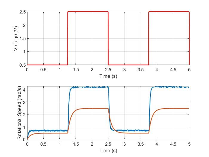
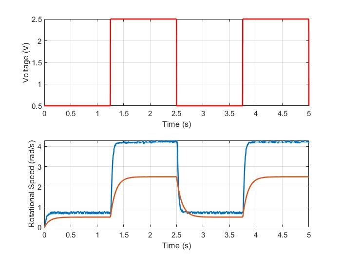
Test multiple (K, τ) combinations in the Simulink model and select the best-fit parameters
Understand how K and τ independently shape the magnitude and speed of a first-order system response

Bump test – voltage and rotational speed vs. time, K=1.53, t=0.0253 — Figure 1: Bump test — voltage and rotational speed vs. time (K=1.53, τ=0.0253)

Figure 2: 63.2% criterion diagram for time constant identification from step response

Equipment & Tools

Quanser SRV02 rotary servo-motor system with gear train
Q2-USB data acquisition board
VoltPAQ power amplifier
MATLAB/Simulink 2020 with QUARC real-time control toolbox
Computer and monitor

Approach & Key Equations

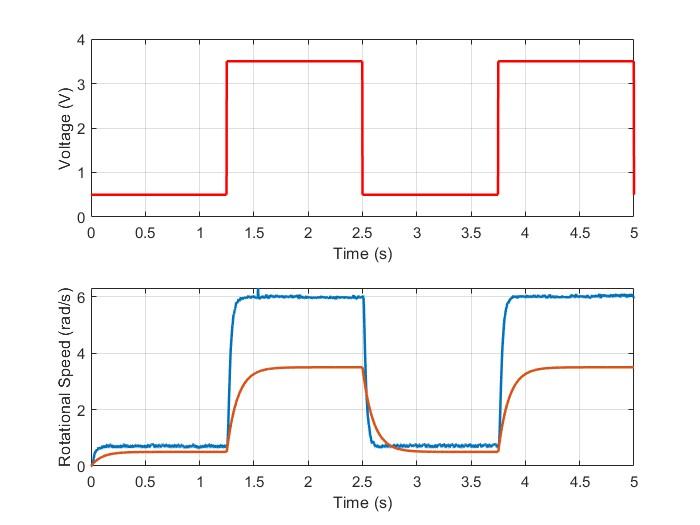
A square-wave voltage (amplitude 1.5 V, offset 2.0 V, frequency 0.4 Hz) was applied to the SRV02 via Simulink’s “Monitor & Tune” mode. The load shaft speed and motor voltage were recorded for 5 seconds. The steady-state gain was computed from the measured speed change divided by the voltage change:

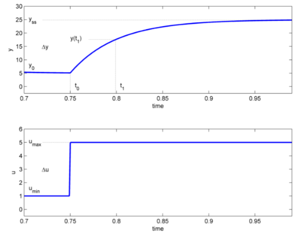
K = (y_ss − y₀) / (u_max − u_min)

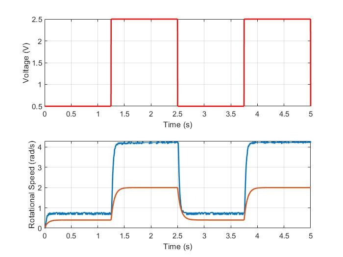
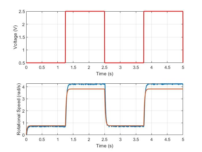
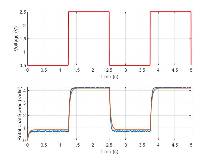
The time constant was identified as the time elapsed between the step onset and the point where the response reached 63.2% of its final steady-state value. Both parameters were then entered into the Simulink model and the simulated output compared visually against the measured response. Multiple (K, τ) pairs were tested until the curves converged.

Model validation iteration – K=1.0, t=0.1, simulated vs. measured speed — Figure 3: Model validation iteration — K=1.0, τ=0.1

Model validation iteration – K=0.8, t=0.06, simulated vs. measured speed — Figure 4: Model validation iteration — K=0.8, τ=0.06

Model validation iteration – K=1.25, t=0.2, simulated vs. measured speed — Figure 5: Model validation iteration — K=1.25, τ=0.2

Key Results

Source	K (rad/s/V)	τ (s)
Nominal (theoretical)	1.53	0.0253
Bump test	1.7866	0.048
Model validation (best fit)	1.68	0.044

K_e,b = (6.051 − 0.691) / (3.5 − 0.5) = 1.787 rad/s/V from the bump test. The time constant τ_e,b = 1.298 − 1.25 = 0.048 s at the 63.2% crossing.
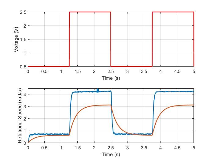
The nominal model (K = 1.53, τ = 0.0253) under-predicted steady-state speed and over-predicted response speed due to parameter uncertainty and unmodeled friction in the gear train.
The validated model (K = 1.68, τ = 0.044) produced near-exact overlay with the measured response, confirming that experimental identification outperforms purely theoretical parameters for real hardware.

Model validation – K=1.53, t=0.0253 (nominal), simulated vs. measured speed — Figure 6: Nominal model (K=1.53, τ=0.0253) — simulated vs. measured

Model validation – K=1.7866, t=0.048 (bump test result), simulated vs. measured speed — Figure 7: Bump test result (K=1.7866, τ=0.048) — simulated vs. measured

Best-fit validated model – K=1.68, t=0.044, near-exact overlay of simulated and measured speed — Figure 8: Best-fit validated model (K=1.68, τ=0.044) — near-exact overlay

MATLAB Code

Data was saved from the Simulink workspace and plotted with subplots showing voltage and load shaft speed. Bump test parameters were read from MATLAB cursor coordinates on the response plot.

% Plot voltage and rotational speed vs time
figure();
subplot(2,1,1)
plot(Vm(:,1), Vm(:,2), 'r', 'LineWidth', 1.5);
xlabel('Time (s)');  ylabel('Voltage (V)');

subplot(2,1,2)
plot(wl(:,1), wl(:,2), 'LineWidth', 1.5);   % measured
hold on
plot(wl(:,1), wl(:,3), 'LineWidth', 1.5);   % simulated
xlabel('Time (s)');  ylabel('Rotational Speed (rad/s)');

% Bump test gain and time constant
K_eb   = (y_ss - y_0) / (u_max - u_min);     % = 1.7866 (rad/s)/V
tau_eb = t_63pct - t_step_onset;             % = 0.048 s

Valuable Takeaways

Experimental system identification is more reliable than purely theoretical models. The nominal model — built from manufacturer specs — was noticeably less accurate than the bump test result, because real hardware includes friction, gear lash, and manufacturing tolerances that no datasheet captures.
K controls “how far” and τ controls “how fast.” Understanding these two parameters independently is the foundation for all subsequent controller design: a smaller τ means faster response but also more sensitivity to noise and model uncertainty.
Model validation is iterative. Overlaying simulation and measurement, then adjusting parameters until they match, is the standard workflow in model-based design — used in aerospace autopilot development, robotics, and automotive control systems.
Gained foundational experience with MATLAB/Simulink hardware-in-the-loop testing and the Quanser QUARC interface — the platform used in ERAU’s flight control and robotics research programs.